14. Fault Tree Uncertainties #

In addition to what’s in Anaconda, this lecture will need the following libraries:

!pip install quantecon tabulate

14.1. Overview #

This lecture puts elementary tools to work to approximate probability distributions of the annual failure rates of a system consisting of a number of critical parts.

We’ll use log normal distributions to approximate probability distributions of critical component parts.

To approximate the probability distribution of the sum of \(n\) lognormal random variables (representing the system’s total failure rate), we compute the convolution of these distributions.

We’ll use the following concepts and tools:

lognormal distributions
the convolution theorem that describes the probability distribution of the sum of independent random variables
fault tree analysis for approximating a failure rate of a multi-component system
a hierarchical probability model for describing uncertain probabilities
Fourier transforms and inverse Fourier transforms as efficient ways of computing convolutions of sequences

14.2. The lognormal distribution #

If random variable \(x\) follows a normal distribution with mean \(\mu\) and variance \(\sigma^2\), then \(y = \exp(x)\) follows a lognormal distribution with parameters \(\mu, \sigma^2\).

Note

We refer to \(\mu\) and \(\sigma^2\) as parameters rather than mean and variance because:

\(\mu\) and \(\sigma^2\) are the mean and variance of \(x = \log(y)\)
They are not the mean and variance of \(y\)
The mean of \(y\) is \(\exp(\mu + \frac{1}{2}\sigma^2)\) and the variance is \((e^{\sigma^2} - 1) e^{2\mu + \sigma^2}\)

A lognormal random variable \(y\) is always nonnegative.

The probability density function for \(y\) is

(14.1)#\[f(y) = \frac{1}{y \sigma \sqrt{2 \pi}} \exp \left( \frac{- (\log y - \mu)^2 }{2 \sigma^2} \right), \quad y \geq 0\]

Important properties of a lognormal random variable are:

(14.2)#\[\begin{split}\begin{aligned} \text{Mean:} & \quad e ^{\mu + \frac{1}{2} \sigma^2} \\ \text{Variance:} & \quad (e^{\sigma^2} - 1) e^{2 \mu + \sigma^2} \\ \text{Median:} & \quad e^\mu \\ \text{Mode:} & \quad e^{\mu - \sigma^2} \\ \text{0.95 quantile:} & \quad e^{\mu + 1.645 \sigma} \\ \text{0.95/0.05 quantile ratio:} & \quad e^{3.29 \sigma} \end{aligned}\end{split}\]

14.2.1. Stability properties#

Recall that independent normally distributed random variables have the following stability property:

If \(x_1 \sim N(\mu_1, \sigma_1^2)\) and \(x_2 \sim N(\mu_2, \sigma_2^2)\) are independent, then \(x_1 + x_2 \sim N(\mu_1 + \mu_2, \sigma_1^2 + \sigma_2^2)\).

Independent lognormal distributions have a different stability property: the product of independent lognormal random variables is also lognormal.

Specifically, if \(y_1\) is lognormal with parameters \((\mu_1, \sigma_1^2)\) and \(y_2\) is lognormal with parameters \((\mu_2, \sigma_2^2)\), then \(y_1 y_2\) is lognormal with parameters \((\mu_1 + \mu_2, \sigma_1^2 + \sigma_2^2)\).

Warning

While the product of two lognormal distributions is lognormal, the sum of two lognormal distributions is not lognormal.

This observation motivates the central challenge of this lecture: approximating the probability distribution of sums of independent lognormal random variables.

14.3. The convolution theorem #

Let \(x\) and \(y\) be independent random variables with probability densities \(f(x)\) and \(g(y)\), where \(x, y \in \mathbb{R}\).

Let \(z = x + y\).

Then the probability density of \(z\) is

(14.3)#\[h(z) = (f * g)(z) \equiv \int_{-\infty}^\infty f(\tau) g(z - \tau) d\tau\]

where \((f*g)\) denotes the convolution of \(f\) and \(g\).

For nonnegative random variables, this specializes to

(14.4)#\[h(z) = (f * g)(z) \equiv \int_{0}^z f(\tau) g(z - \tau) d\tau\]

14.3.1. Discrete convolution#

We will use a discretized version of the convolution formula.

We replace both \(f\) and \(g\) with discretized counterparts, normalized to sum to 1.

The discrete convolution formula is

(14.5)#\[h_n = (f*g)_n = \sum_{m=0}^n f_m g_{n-m}, \quad n \geq 0\]

This computes the probability mass function of the sum of two discrete random variables.

14.3.2. Example: discrete distributions#

Consider two probability mass functions:

\[ f_j = \mathbb{P}\{X = j\}, \quad j = 0, 1 \]

and

\[ g_j = \mathbb{P}\{Y = j\}, \quad j = 0, 1, 2, 3 \]

The distribution of \(Z = X + Y\) is given by the convolution \(h = f * g\).

# Define probability mass functions
f = [0.75, 0.25]
g = [0.0, 0.6, 0.0, 0.4]

# Compute convolution using two methods
h = np.convolve(f, g)
hf = fftconvolve(f, g)

print(f"f = {f}, sum = {np.sum(f):.3f}")
print(f"g = {g}, sum = {np.sum(g):.3f}")
print(f"h = {h}, sum = {np.sum(h):.3f}")
print(f"hf = {hf}, sum = {np.sum(hf):.3f}")

f = [0.75, 0.25], sum = 1.000
g = [0.0, 0.6, 0.0, 0.4], sum = 1.000
h = [0.   0.45 0.15 0.3  0.1 ], sum = 1.000
hf = [0.   0.45 0.15 0.3  0.1 ], sum = 1.000

Both numpy.convolve and scipy.signal.fftconvolve produce the same result, but fftconvolve is much faster for long sequences.

We will use fftconvolve throughout this lecture for efficiency.

14.4. Approximating continuous distributions #

We now verify that discretized distributions can accurately approximate samples from underlying continuous distributions.

We generate samples of size 25,000 from three independent lognormal random variables and compute their pairwise and triple-wise sums.

We then compare histograms of the samples with histograms of the discretized distributions.

# Set parameters for lognormal distributions
μ, σ = 5.0, 1.0
n_samples = 25000

# Generate samples
rng = np.random.default_rng(1234)
s1 = rng.lognormal(μ, σ, n_samples)
s2 = rng.lognormal(μ, σ, n_samples)
s3 = rng.lognormal(μ, σ, n_samples)

# Compute sums
ssum2 = s1 + s2
ssum3 = s1 + s2 + s3

# Plot histogram of s1
fig, ax = plt.subplots()
ax.hist(s1, 1000, density=True, alpha=0.6)
ax.set_xlabel('value')
ax.set_ylabel('density')
plt.show()

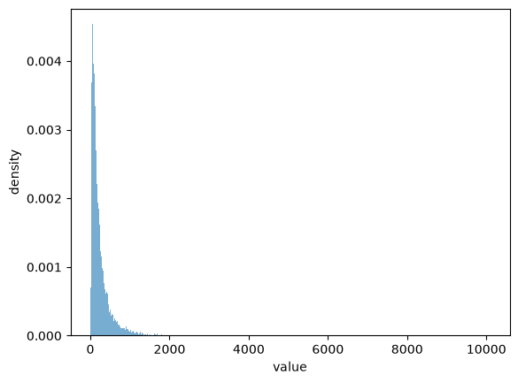
_images/1f9e7e72294307e506e78c0b61ae7f100a56b05def5e7436902e6418e70afbd2.png — Fig. 14.1 Sample histogram of one lognormal#

# Plot histogram of sum of two lognormal distributions
fig, ax = plt.subplots()
ax.hist(ssum2, 1000, density=True, alpha=0.6)
ax.set_xlabel('value')
ax.set_ylabel('density')
plt.show()

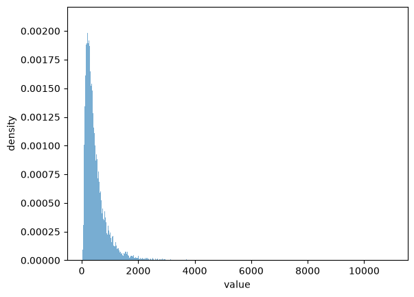
_images/c84ca41e209e8f09d0323cce2ea87b32fa4fca457501b688cfffd4f83fac63b5.png — Fig. 14.2 Histogram of a sum of two lognormals#

# Plot histogram of sum of three lognormal distributions
fig, ax = plt.subplots()
ax.hist(ssum3, 1000, density=True, alpha=0.6)
ax.set_xlabel('value')
ax.set_ylabel('density')
plt.show()

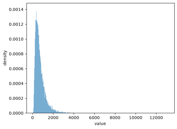
_images/b8185cbbdd3066c468fb7b650eb74222ae9c27b1d6c2cbecd16c7a863d869ba7.png — Fig. 14.3 Histogram of a sum of three lognormals#

Let’s verify that the sample mean matches the theoretical mean:

samp_mean = np.mean(s2)
theoretical_mean = np.exp(μ + σ**2 / 2)

print(f"Theoretical mean: {theoretical_mean:.3f}")
print(f"Sample mean: {samp_mean:.3f}")

Theoretical mean: 244.692
Sample mean: 243.197

14.5. Discretizing the lognormal distribution #

We define helper functions to create discretized versions of lognormal probability density functions.

We write out the density by hand to keep the formula (14.1) in view; scipy.stats.lognorm(s=σ, scale=np.exp(μ)).pdf(x) computes the same thing.

def lognormal_pdf(x, μ, σ):
    """
    Compute lognormal probability density function.
    """
    p = 1 / (σ * x * np.sqrt(2 * np.pi)) \
            * np.exp(-0.5 * ((np.log(x) - μ) / σ)**2)
    return p


def discretize_lognormal(μ, σ, I, m):
    """
    Discretize a lognormal distribution on the grid 0, m, 2m, ..., up to I.

    Parameters
    ----------
    μ, σ : parameters of the lognormal distribution
    I    : upper end of the grid, which truncates the right tail
    m    : spacing between grid points, which sets the resolution

    Returns
    -------
    p_array      : the density evaluated on the grid
    p_array_norm : the implied probability mass function, summing to one
    x            : the grid itself, with I / m points
    """
    x = np.arange(1e-7, I, m)
    p_array = lognormal_pdf(x, μ, σ)
    p_array_norm = p_array / np.sum(p_array)
    return p_array, p_array_norm, x

Two separate choices govern the quality of this approximation, and it pays to keep them straight.

\(I\) fixes where the grid stops, so it controls how much of the right tail we throw away
\(m\) fixes the spacing between grid points, so it controls resolution

The grid has \(I/m\) points, so raising \(I\) at fixed \(m\) buys range, while lowering \(m\) at fixed \(I\) buys accuracy.

Once \(I\) is large enough that almost no probability mass lies beyond it, further increases change nothing, and only \(m\) matters.

Exercise 14.1 asks you to verify this.

Note

scipy.signal.fftconvolve pads its inputs to a convenient length internally, so there is no need to choose \(I/m\) to be a power of two.

# Set grid parameters
p = 15
I = 2**p  # where the grid stops: truncates the right tail
m = 0.1   # spacing between grid points: sets the resolution

Let’s visualize how well the discretized distribution approximates the continuous lognormal distribution:

# Compute discretized PDF
pdf, pdf_norm, x = discretize_lognormal(μ, σ, I, m)

# Plot discretized PDF against histogram
fig, ax = plt.subplots(figsize=(10, 6))
ax.plot(x, pdf, 'r-', lw=2, label='discretized PDF')
ax.hist(s1, 1000, density=True, alpha=0.6, label='sample histogram')
ax.set_xlim(0, 2500)
ax.set_xlabel('value')
ax.set_ylabel('density')
ax.legend()
plt.show()

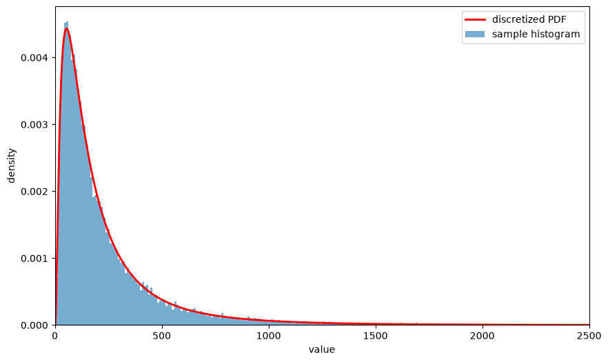
_images/6e48ad081653c3aef63a04db0b75bdefa146008ae01134d1cc07693c79f53e1c.png — Fig. 14.4 Discretized density against sample#

Now let’s verify that the discretized distribution has the correct mean:

# Compute mean from discretized PDF
mean_discrete = np.sum(x * pdf_norm)
mean_theory = np.exp(μ + 0.5 * σ**2)

print(f"Theoretical mean: {mean_theory:.3f}")
print(f"Discretized mean: {mean_discrete:.3f}")

Theoretical mean: 244.692
Discretized mean: 244.691

14.6. Convolving probability mass functions #

Now let’s use the convolution theorem to compute the probability distribution of a sum of the two lognormal random variables we have parameterized above.

We’ll also compute the probability distribution of a sum of three log normal distributions constructed above.

For long sequences, scipy.signal.fftconvolve is much faster than numpy.convolve because it uses fast Fourier transforms.

Let’s define the Fourier transform and the inverse Fourier transform first

14.6.1. The fast Fourier transform#

The Fourier transform of a sequence \(\{x_t\}_{t=0}^{T-1}\) is

(14.6)#\[x(\omega_j) = \sum_{t=0}^{T-1} x_t \exp(-i \omega_j t)\]

where \(\omega_j = \frac{2\pi j}{T}\) for \(j = 0, 1, \ldots, T-1\).

The inverse Fourier transform of the sequence \(\{x(\omega_j)\}_{j=0}^{T-1}\) is

(14.7)#\[x_t = T^{-1} \sum_{j=0}^{T-1} x(\omega_j) \exp(i \omega_j t)\]

The sequences \(\{x_t\}_{t=0}^{T-1}\) and \(\{x(\omega_j)\}_{j=0}^{T-1}\) contain the same information.

The pair of equations (14.6) and (14.7) tell how to recover one series from its Fourier partner.

The program scipy.signal.fftconvolve deploys the theorem that a convolution of two sequences \(\{f_k\}, \{g_k\}\) can be computed in the following way:

Compute Fourier transforms \(F(\omega), G(\omega)\) of the \(\{f_k\}\) and \(\{g_k\}\) sequences, respectively
Form the product \(H (\omega) = F(\omega) G (\omega)\)
The convolution of \(f * g\) is the inverse Fourier transform of \(H(\omega)\)

The fast Fourier transform and the associated inverse fast Fourier transform execute these calculations very quickly.

This is the algorithm used by fftconvolve.

Let’s do a warmup calculation that compares the times taken by numpy.convolve and scipy.signal.fftconvolve

Our three components are identically distributed, so a single discretization serves for all of them.

# Discretize the lognormal distribution; the three components are IID
_, pmf1, x = discretize_lognormal(μ, σ, I, m)
pmf2 = pmf3 = pmf1

# Direct convolution costs O(N²), so we time it on a short prefix
short = pmf1[:20_000]

with qe.Timer() as timer_numpy:
    np.convolve(short, short)
time_numpy = timer_numpy.elapsed

with qe.Timer() as timer_fft:
    fftconvolve(short, short)
time_fft = timer_fft.elapsed

print(f"On {len(short):,} points:")
print(f"  np.convolve: {time_numpy:.4f} seconds")
print(f"  fftconvolve: {time_fft:.4f} seconds")
print(f"  speedup:     {time_numpy / time_fft:.0f}x")

0.0655 seconds elapsed
0.0026 seconds elapsed
On 20,000 points:
  np.convolve: 0.0655 seconds
  fftconvolve: 0.0026 seconds
  speedup:     25x

The gap widens rapidly with the length of the sequences, because direct convolution costs \(O(N^2)\) operations while the FFT approach costs \(O(N \log N)\).

On the full grid used below, the direct method would be far slower still.

# The full calculation, done the fast way
conv_fft = fftconvolve(fftconvolve(pmf1, pmf2), pmf3)
print(f"grid points per component: {len(pmf1):,}")

grid points per component: 327,680

Now let’s plot our computed probability mass function approximation for the sum of two log normal random variables against the histogram of the sample that we formed above

# Compute convolution of two distributions for comparison
conv2 = fftconvolve(pmf1, pmf2)

fig, ax = plt.subplots(figsize=(10, 6))
ax.plot(x, conv2[:len(x)] / m, 'r-', lw=2, label='convolution (FFT)')
ax.hist(ssum2, 1000, density=True, alpha=0.6, label='sample histogram')
ax.set_xlim(0, 5000)
ax.set_xlabel('value')
ax.set_ylabel('density')
ax.legend()
plt.show()

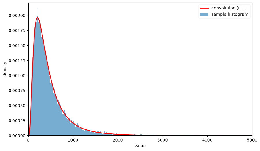
_images/814c8d8da009864aa741730ebc0c20768465111358b87280770c4b27650f0eed.png — Fig. 14.5 Convolution against sample, two components#

Now we present the plot for the sum of three lognormal random variables:

fig, ax = plt.subplots(figsize=(10, 6))
ax.plot(x, conv_fft[:len(x)] / m, 'r-', lw=2, label='convolution (FFT)')
ax.hist(ssum3, 1000, density=True, alpha=0.6, label='sample histogram')
ax.set_xlim(0, 5000)
ax.set_xlabel('value')
ax.set_ylabel('density')
ax.legend()
plt.show()

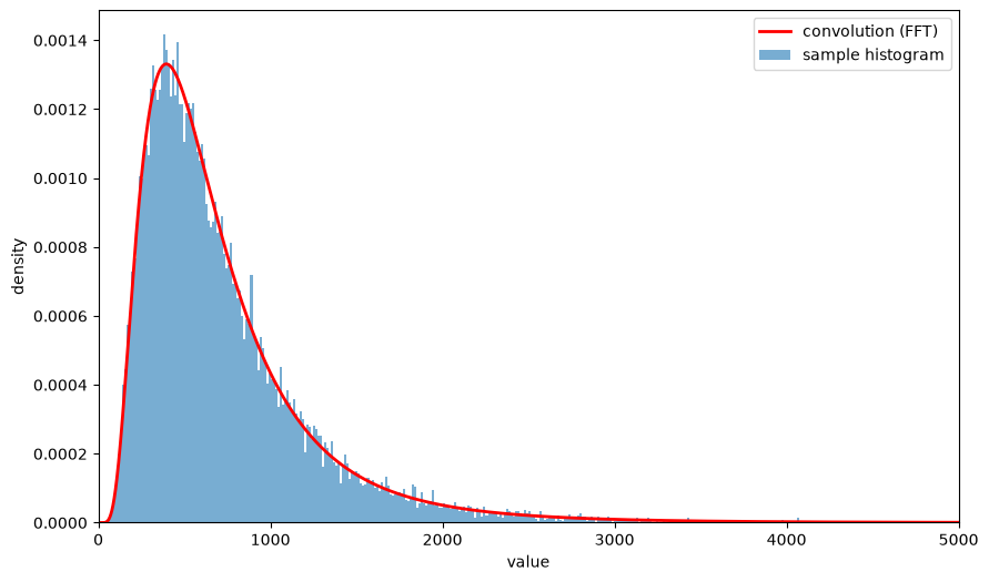
_images/3c3a9825b30300f5d0ffd1b97bc3c7df01d24d4768c3efa4d129cfeab2bb2a4b.png — Fig. 14.6 Convolution against sample, three components#

Let’s verify that the means are correct

# Mean of sum of two distributions
mean_conv2 = np.sum(x * conv2[:len(x)])
mean_theory2 = 2 * np.exp(μ + 0.5 * σ**2)

print(f"Sum of two distributions:")
print(f"  Theoretical mean: {mean_theory2:.3f}")
print(f"  Computed mean: {mean_conv2:.3f}")

Sum of two distributions:
  Theoretical mean: 489.384
  Computed mean: 489.381

# Mean of sum of three distributions
mean_conv3 = np.sum(x * conv_fft[:len(x)])
mean_theory3 = 3 * np.exp(μ + 0.5 * σ**2)

print(f"Sum of three distributions:")
print(f"  Theoretical mean: {mean_theory3:.3f}")
print(f"  Computed mean: {mean_conv3:.3f}")

Sum of three distributions:
  Theoretical mean: 734.076
  Computed mean: 734.071

14.7. Fault tree analysis #

We shall soon apply the convolution theorem to compute the probability of a top event in a failure tree analysis.

Before applying the convolution theorem, we first describe the model that connects constituent events to the top event whose failure rate we seek to quantify.

Fault tree analysis is a widely used technique for assessing system reliability, as described by El-Shanawany et al. [2018].

To construct the statistical model, we repeatedly use what is called the rare event approximation.

14.7.1. The rare event approximation#

We want to compute the probability of an event \(A \cup B\).

For events \(A\) and \(B\), the probability of the union is

\[ P(A \cup B) = P(A) + P(B) - P(A \cap B) \]

where \(A \cup B\) is the event that \(A\) or \(B\) occurs, and \(A \cap B\) is the event that \(A\) and \(B\) both occur.

If \(A\) and \(B\) are independent, then \(P(A \cap B) = P(A) P(B)\).

When \(P(A)\) and \(P(B)\) are both small, \(P(A) P(B)\) is even smaller.

The rare event approximation is

\[ P(A \cup B) \approx P(A) + P(B) \]

This approximation is widely used in system failure analysis.

14.7.2. System failure probability#

Consider a system with \(n\) critical components where system failure occurs when any component fails.

We assume:

The failure probability \(P(A_i)\) of each component \(A_i\) is small
Component failures are statistically independent

We repeatedly apply a rare event approximation to obtain the following formula for the probability of a system failure:

\[ P(F) \approx P(A_1) + P (A_2) + \cdots + P (A_n) \]

(14.8)#\[P(F) \approx \sum_{i=1}^n P(A_i)\]

where \(P(F)\) is the system failure probability.

Probabilities for each event are recorded as failure rates per year.

Note

Strictly speaking, a failure rate per year and a failure probability within a year are different objects.

For rare events they nearly coincide, because \(1 - e^{-\lambda} \approx \lambda\) when \(\lambda\) is small.

The same approximation that lets us add probabilities across components also lets us move between rates and probabilities, so we follow the reliability literature in using the two words interchangeably here.

14.8. Failure rates unknown #

Now we come to the problem that really interests us, following El-Shanawany et al. [2018] and Greenfield and Sargent [1993] in the spirit of Apostolakis [1990].

The component failure rates \(P(A_i)\) are not known precisely and must be estimated.

We address this problem by specifying probabilities of probabilities that capture one notion of not knowing the constituent probabilities that are inputs into a failure tree analysis.

Thus, we assume that a system analyst is uncertain about the failure rates \(P(A_i), i =1, \ldots, n\) for components of a system.

The analyst copes with this situation by regarding the system’s failure probability \(P(F)\) and each of the component probabilities \(P(A_i)\) as random variables.

dispersions of the probability distribution of \(P(A_i)\) characterizes the analyst’s uncertainty about the failure probability \(P(A_i)\)
the dispersion of the implied probability distribution of \(P(F)\) characterizes his uncertainty about the probability of a system’s failure.

This leads to what is sometimes called a hierarchical model in which the analyst has probabilities about the probabilities \(P(A_i)\).

Note

Two distinct kinds of randomness appear in this model, and it is worth keeping them apart.

Aleatory uncertainty is the randomness in whether a component fails during a given year; it is described by the failure rate \(P(A_i)\).

Epistemic uncertainty is the analyst’s ignorance about the value of that rate; it is described by the lognormal distribution that he places over \(P(A_i)\).

The distribution that we compute below is an epistemic object: it describes what the analyst knows about a failure rate, not how often the system fails.

Separating the two is the central recommendation of Apostolakis [1990].

The analyst formalizes his uncertainty by assuming that

the failure probability \(P(A_i)\) is itself a log normal random variable with parameters \((\mu_i, \sigma_i)\).
failure rates \(P(A_i)\) and \(P(A_j)\) are statistically independent for all pairs with \(i \neq j\).

The analyst calibrates the parameters \((\mu_i, \sigma_i)\) for the failure events \(i = 1, \ldots, n\) by reading reliability studies in engineering papers that have studied historical failure rates of components that are as similar as possible to the components being used in the system under study.

The analyst assumes that such information about the observed dispersion of annual failure rates, or times to failure, can inform him of what to expect about parts’ performances in his system.

The analyst assumes that the random variables \(P(A_i)\) are statistically mutually independent.

Warning

Independence is a strong assumption and it is the one that reliability analysts worry about most.

A design flaw, a shared power supply, a common maintenance crew, or a single environmental shock can push many components toward failure at once.

Such common-cause failures make the upper tail of the distribution of \(P(F)\) much fatter than the independent calculation suggests, which is precisely the region that a safety regulator cares about.

Exercise 14.5 quantifies how much difference this makes.

The analyst wants to approximate a probability mass function and cumulative distribution function of the system’s failure probability \(P(F)\).

We say probability mass function because of how we discretize each random variable, as described earlier.

The analyst calculates the probability mass function for the top event \(F\), i.e., a system failure, by repeatedly applying the convolution theorem to compute the probability distribution of a sum of independent log normal random variables, as described in equation (14.8).

14.9. Application: waste hoist failure rate #

We now analyze a real-world example with \(n = 14\) components.

The application estimates the annual failure rate of a critical hoist at a nuclear waste facility.

A regulatory agency requires the system to be designed so that the top event failure rate is small with high probability.

14.9.1. Model specification#

This example is Design Option B-2 (Case I) described in Table 10 on page 27 of Greenfield and Sargent [1993].

The table describes parameters \(\mu_i, \sigma_i\) for fourteen log normal random variables that consist of seven pairs of random variables that are identically and independently distributed.

Within a pair, parameters \(\mu_i, \sigma_i\) are the same
As described in table 10 of Greenfield and Sargent [1993] p. 27, parameters of log normal distributions for the seven unique probabilities \(P(A_i)\) have been calibrated to be the values in the following Python code:

# Component failure rate parameters 
# (see Table 10 of Greenfield & Sargent 1993)
params = [
    (4.28, 1.1947),   # Component type 1
    (3.39, 1.1947),   # Component type 2
    (2.795, 1.1947),  # Component type 3
    (2.717, 1.1947),  # Component type 4
    (2.717, 1.1947),  # Component type 5
    (1.444, 1.4632),  # Component type 6
    (-0.040, 1.4632), # Component type 7 (appears 8 times)
]

Note

Since failure rates are very small, these lognormal distributions actually describe \(P(A_i) \times 10^{-9}\).

So the probabilities that we’ll put on the \(x\) axis of the probability mass function and associated cumulative distribution function should be multiplied by \(10^{-09}\)

We define a helper function to find array indices:

def find_nearest(array, value):
    """
    Index of the array element nearest to the given value.

    Applied to a cumulative distribution function, this returns the grid point
    whose cumulative probability is closest to a target, which for a finely
    discretized distribution is indistinguishable from the usual definition of
    a quantile as the smallest x with CDF(x) >= q.
    """
    array = np.asarray(array)
    idx = (np.abs(array - value)).argmin()
    return idx

We compute the required thirteen convolutions in the following code.

(Please feel free to try different values of the power parameter \(p\) that we use to set the number of points in our grid for constructing the probability mass functions that discretize the continuous log normal distributions.)

# Set grid parameters
p = 15
I = 2**p
m = 0.05

# Discretize all component failure rate distributions
# First 6 components use unique parameters, last 8 share the same parameters
component_pmfs = []
for μ, σ in params[:6]:
    _, pmf, x = discretize_lognormal(μ, σ, I, m)
    component_pmfs.append(pmf)

# Add 8 copies of component type 7
μ7, σ7 = params[6]
_, pmf7, x = discretize_lognormal(μ7, σ7, I, m)
component_pmfs.extend([pmf7] * 8)

# Compute system failure distribution via sequential convolution
with qe.Timer() as timer:
    system_pmf = component_pmfs[0]
    for pmf in component_pmfs[1:]:
        system_pmf = fftconvolve(system_pmf, pmf)

print(f"Time for 13 convolutions: {timer.elapsed:.4f} seconds")

# the convolution lives on the same grid spacing, but extends much further
system_grid = np.arange(len(system_pmf)) * m
print(f"grid points in the answer: {len(system_pmf):,}")

7.5745 seconds elapsed
Time for 13 convolutions: 7.5745 seconds
grid points in the answer: 9,175,027

Before plotting the cumulative distribution function, let’s look at the density itself.

fig, ax = plt.subplots(figsize=(10, 6))
upper = 2000
ax.plot(system_grid[:int(upper/m)], system_pmf[:int(upper/m)] / m, 'b-', lw=2)
ax.set_xlabel(r'failure rate ($\times 10^{-9}$ per year)')
ax.set_ylabel('density')
plt.show()

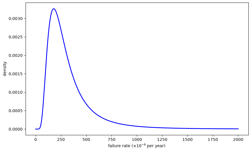
_images/1d4c092094ca93f790d54331b8d8957dd2a8512fd56cd3466b1bbcfb66da0bac.png — Fig. 14.7 Density of the system failure rate#

The density is strongly skewed to the right: a long upper tail stretches far beyond the bulk of the distribution.

This asymmetry is what makes a single point estimate of a failure rate a poor summary, and it is why the analyst reports quantiles instead.

We now plot a counterpart to the cumulative distribution function (CDF) in figure 5 on page 29 of Greenfield and Sargent [1993]

# Compute cumulative distribution function
cdf = np.cumsum(system_pmf)

# Plot CDF
Nx = 1400
fig, ax = plt.subplots(figsize=(10, 6))
ax.plot(x[:int(Nx / m)], cdf[:int(Nx / m)], 'b-', lw=2)

# Add reference lines for key quantiles
quantile_levels = [0.05, 0.10, 0.50, 0.90, 0.95]
for q in quantile_levels:
    ax.axhline(q, color='gray', linestyle='--', alpha=0.5)

ax.set_xlim(0, Nx)
ax.set_ylim(0, 1)
ax.set_xlabel(r'failure rate ($\times 10^{-9}$ per year)')
ax.set_ylabel('cumulative probability')
plt.show()

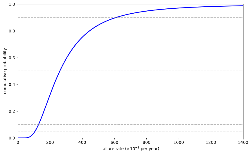
_images/e76d46cd188f184bb0156391fc63ab436a76d7f0ca33eadf20bf76ee21d21a8b.png — Fig. 14.8 CDF of the system failure rate#

We also present a counterpart to their Table 11 on page 28 of Greenfield and Sargent [1993], which lists key quantiles of the system failure rate distribution

# Percentiles reported in Table 11 of Greenfield and Sargent (1993),
# together with their published values, in units of 10^-9 per year
reference = {1.0: 77, 10.0: 130, 50.0: 263, 66.5: 341,
             85.0: 513, 95.0: 811, 99.0: 1480, 99.78: 2490}

table_data = []
for pc, published in reference.items():
    ours = system_grid[find_nearest(cdf, pc/100)]
    table_data.append([f"{pc}%", f"{ours:.1f}", published,
                       f"{100*(ours - published)/published:+.1f}%"])

print("\nSystem failure rate quantiles (×10^-9 per year):")
print(tabulate(table_data,
      headers=['Percentile', 'Computed here', 'Greenfield-Sargent', 'Difference'],
      tablefmt='grid'))

System failure rate quantiles (×10^-9 per year):
+--------------+-----------------+----------------------+--------------+
| Percentile   |   Computed here |   Greenfield-Sargent | Difference   |
+==============+=================+======================+==============+
| 1.0%         |            76.2 |                   77 | -1.1%        |
+--------------+-----------------+----------------------+--------------+
| 10.0%        |           128.2 |                  130 | -1.4%        |
+--------------+-----------------+----------------------+--------------+
| 50.0%        |           260.6 |                  263 | -0.9%        |
+--------------+-----------------+----------------------+--------------+
| 66.5%        |           338.6 |                  341 | -0.7%        |
+--------------+-----------------+----------------------+--------------+
| 85.0%        |           509.4 |                  513 | -0.7%        |
+--------------+-----------------+----------------------+--------------+
| 95.0%        |           807.6 |                  811 | -0.4%        |
+--------------+-----------------+----------------------+--------------+
| 99.0%        |          1470.2 |                 1480 | -0.7%        |
+--------------+-----------------+----------------------+--------------+
| 99.78%       |          2474.9 |                 2490 | -0.6%        |
+--------------+-----------------+----------------------+--------------+

Our quantiles reproduce the published ones to within one and a half per cent, and slightly understate each of them.

The small discrepancies reflect the precision of the reported parameters \(\mu_i, \sigma_i\), the grid spacing \(m\), and the point at which the grid is truncated.

14.9.2. Reading the answer#

The numbers in this table, rather than any single one of them, are the output of the analysis.

The median failure rate is about \(261 \times 10^{-9}\) per year, while the 95th percentile is about \(808 \times 10^{-9}\), three times larger.

That spread is not a statement about how often the hoist fails; it is a statement about how little the analyst knows about how often the hoist fails.

Notice also where the mean of the distribution falls.

mean_rate = np.sum(system_grid * system_pmf)
mean_percentile = 100 * cdf[find_nearest(system_grid, mean_rate)]

print(f"mean failure rate: {mean_rate:.1f} × 10⁻⁹ per year")
print(f"the mean sits at the {mean_percentile:.1f}th percentile")

mean failure rate: 338.1 × 10⁻⁹ per year
the mean sits at the 66.4th percentile

Because the distribution is skewed, the mean lies well above the median, at about the 66th percentile.

This is why Table 11 of Greenfield and Sargent [1993] records the mean alongside the 66.5th percentile.

The practical implication is the one that motivated the original study.

# The point estimate used in the U.S. Department of Energy's 1990 risk
# assessment, expressed in the same units
doe_estimate = 220    # 2.2 × 10^-7 per year

pct = 100 * cdf[find_nearest(system_grid, doe_estimate)]
print(f"the DOE point estimate of {doe_estimate} × 10⁻⁹ lies at "
      f"the {pct:.0f}th percentile")
print(f"so the analyst assigns probability {100-pct:.0f}% to the "
      f"true rate exceeding it")

the DOE point estimate of 220 × 10⁻⁹ lies at the 39th percentile
so the analyst assigns probability 61% to the true rate exceeding it

An analysis that reports a single number in place of a distribution conveys none of this.

Greenfield and Sargent [1993] made exactly this point: reading their figure, they put the Department of Energy’s point estimate at the 36th percentile and concluded that there was roughly a 64 per cent chance that the true failure rate was higher.

14.10. Exercises #

Exercise 14.1

Our discretization involves two separate choices: where the grid stops, \(I = 2^p\), and how finely it is spaced, \(m\).

Investigate what each one controls.

Holding \(m = 0.05\) fixed, compute the median, the 95th percentile and the 99.78th percentile of the system failure rate for \(p = 10, 11, \ldots, 15\). For each \(p\), also compute how much probability mass the truncation discards, using \(\sum_i \mathbb{P}\{P(A_i) > I\}\).
Holding \(p = 14\) fixed, repeat for \(m = 0.4, 0.2, 0.1, 0.05, 0.025\).
Which statistic is sensitive to which choice, and why? Are the values \(p = 15\), \(m = 0.05\) used in the lecture well chosen?

Solution

from scipy.stats import norm

def system_distribution(p_grid, m_grid):
    "Failure rate distribution of the whole system on a given grid."
    I_grid = 2**p_grid
    pmfs = []
    for μ_i, σ_i in params[:6]:
        _, pmf_i, _ = discretize_lognormal(μ_i, σ_i, I_grid, m_grid)
        pmfs.append(pmf_i)
    μ7, σ7 = params[6]
    _, pmf7, _ = discretize_lognormal(μ7, σ7, I_grid, m_grid)
    pmfs.extend([pmf7] * 8)

    total = pmfs[0]
    for pmf_i in pmfs[1:]:
        total = fftconvolve(total, pmf_i)
    return total, np.arange(len(total)) * m_grid


def quantiles_of(pmf, grid, levels=(0.5, 0.95, 0.9978)):
    cdf_local = np.cumsum(pmf)
    return [grid[find_nearest(cdf_local, q)] for q in levels]


def discarded_mass(I_grid):
    "Probability that a component's rate exceeds the end of the grid."
    lost = sum(norm.sf((np.log(I_grid) - μ_i)/σ_i) for μ_i, σ_i in params[:6])
    μ7, σ7 = params[6]
    return lost + 8 * norm.sf((np.log(I_grid) - μ7)/σ7)


rows = []
for p_test in range(10, 16):
    pmf_t, grid_t = system_distribution(p_test, 0.05)
    med, q95, q9978 = quantiles_of(pmf_t, grid_t)
    rows.append([p_test, 2**p_test, f"{discarded_mass(2**p_test):.1e}",
                 f"{med:.2f}", f"{q95:.2f}", f"{q9978:.2f}"])

print(tabulate(rows, headers=['p', 'I', 'mass discarded',
                              'median', '95th', '99.78th'], tablefmt='grid'))

+-----+-------+------------------+----------+--------+-----------+
|   p |     I |   mass discarded |   median |   95th |   99.78th |
+=====+=======+==================+==========+========+===========+
|  10 |  1024 |          0.016   |   257.55 | 728.8  |   1247.95 |
+-----+-------+------------------+----------+--------+-----------+
|  11 |  2048 |          0.0028  |   260    | 791.1  |   1870.75 |
+-----+-------+------------------+----------+--------+-----------+
|  12 |  4096 |          0.00039 |   260.5  | 805.3  |   2344.85 |
+-----+-------+------------------+----------+--------+-----------+
|  13 |  8192 |          3.9e-05 |   260.55 | 807.35 |   2460.5  |
+-----+-------+------------------+----------+--------+-----------+
|  14 | 16384 |          2.9e-06 |   260.55 | 807.6  |   2473.85 |
+-----+-------+------------------+----------+--------+-----------+
|  15 | 32768 |          1.6e-07 |   260.55 | 807.6  |   2474.85 |
+-----+-------+------------------+----------+--------+-----------+

rows = []
for m_test in (0.4, 0.2, 0.1, 0.05, 0.025):
    pmf_t, grid_t = system_distribution(14, m_test)
    med, q95, q9978 = quantiles_of(pmf_t, grid_t)
    rows.append([m_test, len(grid_t), f"{med:.3f}", f"{q95:.2f}", f"{q9978:.2f}"])

print(tabulate(rows, headers=['m', 'grid points', 'median', '95th', '99.78th'],
               tablefmt='grid'))

+-------+---------------+----------+--------+-----------+
|     m |   grid points |   median |   95th |   99.78th |
+=======+===============+==========+========+===========+
| 0.4   |        573427 |  264.4   |  811.6 |   2477.6  |
+-------+---------------+----------+--------+-----------+
| 0.2   |       1146867 |  261.8   |  809   |   2475.2  |
+-------+---------------+----------+--------+-----------+
| 0.1   |       2293747 |  260.9   |  807.9 |   2474.2  |
+-------+---------------+----------+--------+-----------+
| 0.05  |       4587507 |  260.55  |  807.6 |   2473.85 |
+-------+---------------+----------+--------+-----------+
| 0.025 |       9175027 |  260.475 |  807.5 |   2473.75 |
+-------+---------------+----------+--------+-----------+

The two choices do quite different jobs.

Truncation governs the far tail.

At \(p = 10\) the 99.78th percentile is badly understated, and it keeps rising until about \(p = 14\), by which point the discarded mass has fallen to roughly \(10^{-6}\).

The median, by contrast, has settled by \(p = 12\): throwing away the extreme right tail of each component hardly moves the middle of the distribution of their sum.

Resolution governs overall precision.

Halving \(m\) shifts every quantile slightly and uniformly, and the shifts are small: going from \(m = 0.4\) to \(m = 0.025\) moves the median by about 1.5 per cent.

The lecture’s choices are sensible.

With \(p = 15\) the discarded mass is around \(10^{-7}\), so even the 99.78th percentile is accurate, and \(m = 0.05\) is fine enough that further refinement changes little.

The moral is that a grid that looks adequate for the median can be badly inadequate for the upper tail, which is exactly the region a safety regulator cares about.

Exercise 14.2

The rare event approximation replaces \(P(A \cup B)\) by \(P(A) + P(B)\), discarding \(P(A \cap B)\).

Assess how good it is here.

Using the mean failure rate of each of the fourteen components as a representative value, compare \(\sum_i p_i\) with the exact probability that at least one component fails, \(1 - \prod_i (1 - p_i)\).
Repeat with all the rates multiplied by \(10^3\), \(10^6\) and \(10^7\), and report the relative error in each case.
At what order of magnitude does the approximation start to matter?

Solution

# representative rate for each of the 14 components
component_means = [np.exp(μ_i + 0.5*σ_i**2) for μ_i, σ_i in params[:6]]
μ7, σ7 = params[6]
component_means.extend([np.exp(μ7 + 0.5*σ7**2)] * 8)
component_means = np.array(component_means)

rows = []
for factor, label in ((1e-9, 'as calibrated'), (1e-6, '× 10³'),
                      (1e-3, '× 10⁶'), (1e-2, '× 10⁷')):
    probs = component_means * factor
    approx = probs.sum()
    exact = 1 - np.prod(1 - probs)
    rows.append([label, f"{approx:.6e}", f"{exact:.6e}",
                 f"{100*(approx - exact)/exact:.4f}%"])

print(tabulate(rows, headers=['failure rates', 'Σ pᵢ', '1 - Π(1-pᵢ)',
                              'relative error'], tablefmt='grid'))

+-----------------+-------------+---------------+------------------+
| failure rates   |        Σ pᵢ |   1 - Π(1-pᵢ) | relative error   |
+=================+=============+===============+==================+
| as calibrated   | 3.38012e-07 |   3.38012e-07 | 0.0000%          |
+-----------------+-------------+---------------+------------------+
| × 10³           | 0.000338012 |   0.000337969 | 0.0127%          |
+-----------------+-------------+---------------+------------------+
| × 10⁶           | 0.338012    |   0.297883    | 13.4715%         |
+-----------------+-------------+---------------+------------------+
| × 10⁷           | 3.38012     |   1.04157     | 224.5216%        |
+-----------------+-------------+---------------+------------------+

At the calibrated magnitudes, around \(3 \times 10^{-7}\) per year in total, the approximation is exact to the precision shown: the neglected term is of order \(p_i p_j \approx 10^{-14}\).

Multiplying every rate by a thousand still leaves an error of about one part in ten thousand.

The approximation only becomes consequential once individual failure probabilities reach the order of a per cent, where it overstates the system failure probability by more than ten per cent, and it fails completely when \(\sum_i p_i\) approaches or exceeds one, where it can return a “probability” greater than one.

Note that a naive check of this approximation – comparing the mean of the computed distribution of \(\sum_i P(A_i)\) with the sum of the component means – reveals nothing, because those two quantities are equal by linearity of expectation whatever the quality of the approximation.

Exercise 14.3

A regulator who learns that the 95th percentile of the failure rate is too high will ask which components to improve.

Answer that question by computing, for each of the seven component types, the 95th percentile of the system failure rate when that type is removed from the system entirely.

Rank the component types by how much they contribute to the upper tail, and compare the ranking with the components’ mean failure rates.

Solution

def system_without(drop):
    "System failure rate distribution with component type `drop` removed."
    pmfs = []
    for k, (μ_i, σ_i) in enumerate(params[:6]):
        if k == drop:
            continue
        _, pmf_i, _ = discretize_lognormal(μ_i, σ_i, I, m)
        pmfs.append(pmf_i)
    if drop != 6:
        μ7, σ7 = params[6]
        _, pmf7, _ = discretize_lognormal(μ7, σ7, I, m)
        pmfs.extend([pmf7] * 8)

    total = pmfs[0]
    for pmf_i in pmfs[1:]:
        total = fftconvolve(total, pmf_i)
    return total, np.arange(len(total)) * m


base_q95 = system_grid[find_nearest(cdf, 0.95)]

rows = []
for k in range(7):
    pmf_k, grid_k = system_without(k)
    q95 = grid_k[find_nearest(np.cumsum(pmf_k), 0.95)]
    μ_k, σ_k = params[k]
    n_units = 8 if k == 6 else 1
    rows.append([f"type {k+1}", n_units, f"{np.exp(μ_k + 0.5*σ_k**2):.1f}",
                 f"{q95:.1f}", f"{100*(base_q95 - q95)/base_q95:.1f}%"])

rows.sort(key=lambda r: -float(r[4].rstrip('%')))
print(f"95th percentile with all components: {base_q95:.1f}\n")
print(tabulate(rows, headers=['removed', 'units', 'mean rate each',
                              '95th pct without it', 'reduction'],
               tablefmt='grid'))

95th percentile with all components: 807.6

+-----------+---------+------------------+-----------------------+-------------+
| removed   |   units |   mean rate each |   95th pct without it | reduction   |
+===========+=========+==================+=======================+=============+
| type 1    |       1 |            147.5 |                 439.3 | 45.6%       |
+-----------+---------+------------------+-----------------------+-------------+
| type 2    |       1 |             60.6 |                 699.4 | 13.4%       |
+-----------+---------+------------------+-----------------------+-------------+
| type 3    |       1 |             33.4 |                 760.1 | 5.9%        |
+-----------+---------+------------------+-----------------------+-------------+
| type 4    |       1 |             30.9 |                 764.7 | 5.3%        |
+-----------+---------+------------------+-----------------------+-------------+
| type 5    |       1 |             30.9 |                 764.7 | 5.3%        |
+-----------+---------+------------------+-----------------------+-------------+
| type 7    |       8 |              2.8 |                 783.7 | 3.0%        |
+-----------+---------+------------------+-----------------------+-------------+
| type 6    |       1 |             12.4 |                 791.1 | 2.0%        |
+-----------+---------+------------------+-----------------------+-------------+

Component type 1 dominates: removing that single unit cuts the 95th percentile by almost half, far more than any other change available to the designer.

The ranking follows the components’ mean rates closely here, because all seven types have similar dispersions.

It need not do so in general: a component with a modest mean but a large \(\sigma\) contributes disproportionately to the upper tail, which is why the analyst works with the whole distribution rather than with means.

Note also that type 7, which appears eight times, matters less than type 1, which appears once.

Counting components is no guide to where the risk lies.

Exercise 14.4

We could have computed the distribution of the system failure rate by simulation instead of by convolution.

Draw samples of all fourteen component rates, sum them, and compare the resulting quantiles with those from the convolution, for sample sizes \(10^4\), \(10^5\) and \(10^6\).

Compare the median, the 95th percentile and the 99.78th percentile.

Which method would you prefer, and why?

Solution

all_params = list(params[:6]) + [params[6]] * 8
rng_mc = np.random.default_rng(0)
levels = (50, 95, 99.78)

rows = []
for N in (10_000, 100_000, 1_000_000):
    draws = sum(rng_mc.lognormal(μ_i, σ_i, N) for μ_i, σ_i in all_params)
    rows.append([f"{N:,}"] + [f"{np.percentile(draws, pc):.1f}" for pc in levels])

rows.append(['convolution'] +
            [f"{system_grid[find_nearest(cdf, pc/100)]:.1f}" for pc in levels])

print(tabulate(rows, headers=['method', 'median', '95th', '99.78th'],
               tablefmt='grid'))

+-------------+----------+--------+-----------+
| method      |   median |   95th |   99.78th |
+=============+==========+========+===========+
| 10,000      |    262.7 |  811.8 |    2240.6 |
+-------------+----------+--------+-----------+
| 100,000     |    261.1 |  807.1 |    2458.4 |
+-------------+----------+--------+-----------+
| 1,000,000   |    260.4 |  807.5 |    2447   |
+-------------+----------+--------+-----------+
| convolution |    260.6 |  807.6 |    2474.9 |
+-------------+----------+--------+-----------+

Simulation converges to the same answer, which is a useful check on both calculations.

The two methods differ in where their errors lie.

Monte Carlo error is largest exactly where the analysis matters most: the 99.78th percentile is pinned down by roughly one draw in five hundred, so with \(10^4\) draws only about twenty observations inform it, and the estimate is visibly off.

The convolution, by contrast, computes the whole distribution at once and its error comes from the grid rather than from sampling noise, so it is equally accurate in the tail as in the middle.

It is also deterministic: the answer does not change when you rerun it with a different seed.

Exercise 14.5

The entire calculation assumes that the fourteen component failure rates are statistically independent.

Investigate what happens when they are not.

Suppose that

\[ \log P(A_i) = \mu_i + \sigma_i \left( \sqrt{\rho}\, z_0 + \sqrt{1-\rho}\, z_i \right), \]

where \(z_0\) is a shock common to all components and \(z_1, \ldots, z_{14}\) are idiosyncratic, all standard normal.

Each component still has exactly its original marginal distribution, but any two of them now have correlation \(\rho\) in logs.

Simulate the system failure rate for \(\rho = 0, 0.2, 0.5, 0.8\) and report the median, the 95th, the 99th and the 99.9th percentiles.

Explain what happens and why it matters for a safety analysis.

Solution

μ_vec = np.array([q[0] for q in all_params])
σ_vec = np.array([q[1] for q in all_params])

N_sim = 400_000
rng_cc = np.random.default_rng(1)

rows = []
for ρ in (0.0, 0.2, 0.5, 0.8):
    z0 = rng_cc.normal(size=(N_sim, 1))
    zi = rng_cc.normal(size=(N_sim, len(all_params)))
    logs = μ_vec + σ_vec * (np.sqrt(ρ)*z0 + np.sqrt(1-ρ)*zi)
    totals = np.exp(logs).sum(axis=1)
    rows.append([ρ] + [f"{np.percentile(totals, pc):.0f}"
                       for pc in (50, 95, 99, 99.9)])

print(tabulate(rows, headers=['ρ', 'median', '95th', '99th', '99.9th'],
               tablefmt='grid'))

+-----+----------+--------+--------+----------+
|   ρ |   median |   95th |   99th |   99.9th |
+=====+==========+========+========+==========+
| 0   |      261 |    811 |   1481 |     3235 |
+-----+----------+--------+--------+----------+
| 0.2 |      242 |    910 |   1650 |     3416 |
+-----+----------+--------+--------+----------+
| 0.5 |      209 |   1043 |   2074 |     4396 |
+-----+----------+--------+--------+----------+
| 0.8 |      179 |   1136 |   2444 |     5763 |
+-----+----------+--------+--------+----------+

Correlation leaves each component’s marginal distribution untouched, and it leaves the mean of the sum untouched as well.

What it changes is the shape of the distribution of the sum.

With independent components, a high draw for one is typically offset by ordinary draws for the others, and the fourteen-fold averaging produces a relatively concentrated total.

A common shock removes that diversification: when \(z_0\) is large every component is bad at once.

The result is a distribution with a lower median and a much heavier upper tail.

At \(\rho = 0.8\) the median falls by about a third while the 99.9th percentile rises by roughly three quarters.

For a safety analysis this is the dangerous direction of error.

Assuming independence when a common cause is present makes the system look both typically safer and much less likely to suffer a very bad year than it really is.

This is why reliability studies devote so much attention to identifying shared power supplies, shared maintenance procedures, common design faults, and other mechanisms that defeat the independence assumption.